Quick Sort Algorithm with example | Step-by-Step Guide

What is Quick Sort?

Quick sort, also known as partition-exchange sort, is an in-place sorting algorithm.

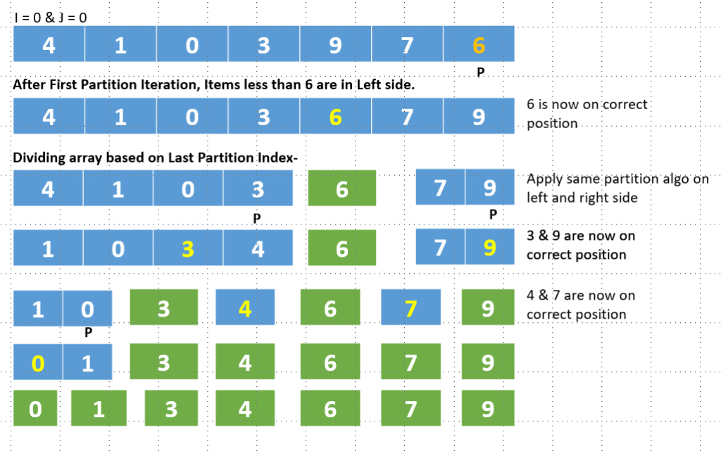
It is a divide-and-conquer algorithm that works on the idea of selecting a pivot element and dividing the array into two subarrays around that pivot.

Every time a quick sort is performed, the selected pivot element is positioned in the appropriate location within the sorted array. By doing this, it is ensured that each pivot element is in the proper sorted position.

With each iteration of quick sort, the problem reduces by 2 steps making quick sort a faster way to sort an array.

One interesting thing to note here is that we can choose any element as our pivot, be it the first element, the last element, or any random element from the array.

💡 Before Understanding sorting algo, First, solve the below problem that is the start of quick sort.

✔️ Separate the elements in two partitions so that all elements smaller than x should be in the Left and all elements greater than x should be in the right position. It is not necessary that x is present in the array. x is just a partition point.

Input  = [4, 1, 0, 3, 9, 7, 6]
X = 4

Output = [1, 0, 3, 4, 9, 7, 6]

We will solve this problem using two-pointer and swapping techniques.

First Pointer (i) => It will run for all array elements. 0 to last index.

Second Pointer (j) => This pointer will also start from index 0. When the I th element is less than the X (given in the problem), We will swap A[i] to A[j] and then only increase the j pointer to the next.

Input  = [4, 1, 0, 3, 9, 7, 6]
X = 4

Start from i = 0 && j = 0

A[0] < X => 4 < 4 => NO => No swapping. Only Increase i by 1.

i = 1 && j  = 0 
A[1] < X => 1 < 4 => TRUE => Swap A[i] to A[j] and Increase J by 1.

[1, 4, 0, 3, 9, 7, 6]

i = 2 && j = 1

A[2] < X => 0 < 4 => TRUE. Swap A[2] to A[1] and increase j.

[1, 0, 4, 3, 9, 7, 6]

i = 3 && j = 2

A[3] < X => 3 < 4 => TRUE => Swap A[3] to A[2] and Increase j.

[1, 4, 3, 0, 9, 7, 6]

 i = 4 && j = 3

A[4] < X => 9 < 4 => FALSE.

i = 5 && j = 3

A[5] < X => 7 < 6 => FALSE.

i = 6 && j = 3

A[6] < X => 6 < 4 => FALSE.

[1, 4, 3, 0, 9, 7, 6]

Now Ending For loop. We can see that 1 4 3 0 are together and 9 7 6 are together.
We were arranging smaller elements than 4 in left side. Now 4 will be swapped
with last smaller element and that is currently on jth value 3.

Swap  X with A[j] => Swap 4 with A[3] => Swap 4 with 0

[1, 0, 3, 4, 9, 7, 6]

Quick Sort
Time complexity – O(nlogn(n)) && Space complexity – O(n)

function quickSort(A) {

    function partition(A, start, end) {
        let pivot = A[end]; // Generally we consider last element as Pivot
        let j = start; // left pointer

        // i < end not <= end. Because last element already taken as Pivot element.
        for (let i = start; i < end; i++) {
            if (A[i] < pivot) {
                [A[j], A[i]] = [A[i], A[j]]; // swap when element is less then pivot element.
                j++; // increase pointer
            }
        }

        /*Now all smaller elements from pivot is in left side so position where
smaller elements ends that position will be of that pivot element. Thats why
simply swapping pivot element with last jth index. */

        [A[j], A[end]] = [A[end], A[j]];
        return j; // pivot index

    }

    function sort(A, start, end) {
        if (start >= end) { // when single element remains in subproblem
            return;
        }
        let pivotIndex = partition(A, start, end);
        sort(A, start, pivotIndex - 1); // apply same partitions and swapping on Left side.
        sort(A, pivotIndex + 1, end); // apply same partitions and swapping on Right side.
    }

    sort(A, 0, A.length - 1);
    return A;
}

More details
https://www.scaler.com/topics/data-structures/quick-sort-algorithm/

QuickSort Algorithm In JavaScript

Time & Space Complexity Of Quick sort

                    n
                /       \
        n/2                      n/2
        / \                       /\
    n/4      n/4             n/4        n/4
    /\        /\              /\         /\
n/8  n/8   n/8 n/8       n/8  n/8     n/8  n/8
..     ..           ..              ..
..      ..          ..              ..

At each step, n is divided by 2 and values are 2^1, 2^2, 2^3, 2 ^4……

So to reach 1, Suppose the steps required is k. It means we can write-

n / 2^k = 1

k = log(n) base 2.

log(n) is required for dividing an array into single elements.

Also, the time complexity of the partition() function would be equal to O(n). This is because, under the function, we are iterating over the array to swap rearranging the array around the pivot element.

So Total Time Complexity of the quick sort algorithm is O(nlogn).

The Space complexity of quick sort is determined by the amount of recursion stack space needed. Because n recursive calls are made in the worst situation, the space complexity is O(n) in that scenario. Additionally, a quick sort algorithm’s average space complexity is O(logn).

JS Mount

Learn More

Quick Sort Algorithm with example | Step-by-Step Guide

What is Quick Sort?

✔️ Separate the elements in two partitions so that all elements smaller than x should be in the Left and all elements greater than x should be in the right position. It is not necessary that x is present in the array. x is just a partition point.

One thought on “Quick Sort Algorithm with example | Step-by-Step Guide”

land rover engine

Leave a Reply Cancel Reply